
A noise-corrected metric for evaluating spatial transcriptomics predicted from histology
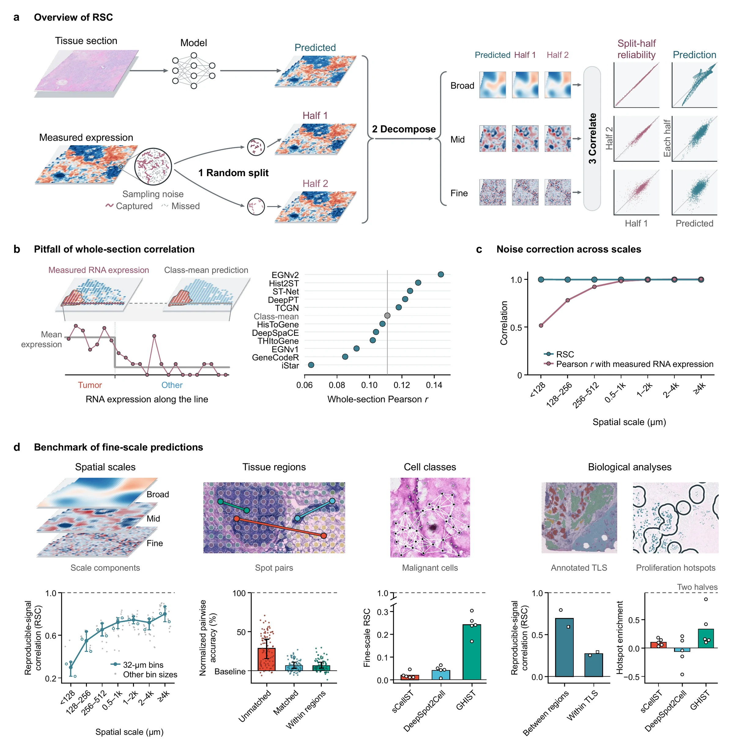
Expression predicted from H&E-stained sections is usually scored by correlation over whole sections. That score rewards a model for recognizing broad tissue regions: in HER2ST, a class-mean baseline that gives every spot of a region the same value reaches Pearson r = 0.111, above the median of 11 published methods (0.108). At fine scales the error runs the other way, because sparse RNA counts carry sampling noise that no prediction can reproduce, and Pearson r with the measured RNA expression understates prediction quality.
The reproducible-signal correlation (RSC) splits the measured RNA molecules at random into two halves. Both halves share the expected expression and carry independent sampling noise. At each spatial scale, and within tissue regions or cell classes, RSC scores a prediction against the signal the two halves share: 1 when the prediction accounts for all reproducible variation at that scale, 0 for chance agreement. RSC is inspired by Fourier shell correlation in cryo-electron microscopy, which compares two half-maps of the same structure.
Even a prediction equal to the underlying expression reaches a Pearson r with measured RNA expression of only 0.44 to 0.57 at the finest scale. Its RSC there is 0.997.
Removing molecules at random lowers whole-section Pearson r from 0.509 to 0.408, while fine-scale RSC changes from 0.337 to 0.386.
How RSC is computed
Split
For each gene and each bin, spot or cell with count N, draw NA ~ Binomial(N, 0.5) and set NB = N − NA. The split is made on raw counts, before any normalization.
Decompose
Transform and center both halves, center and scale the prediction by gene, and take all three apart into spatial scales: a Fourier basis on a regular grid, the eigenvectors of a neighbor-graph Laplacian on spots, diffusion operators on a cell graph.
Correlate
At each scale b, sum over all genes and locations the mean covariance C of the prediction with the two halves, the variance Vmodel of the prediction and the covariance VRNA between the halves. Repeat over independent splits and average.
RSCb = C / √(Vmodel · VRNA)
VRNA estimates the variance of the reproducible signal. The correlation between the two halves, VRNA/√(VAVB), is the split-half reliability ρb. For halves of equal variance, the Pearson r of a prediction with the mean of the halves is RSCb · √(2ρb/(1 + ρb)), so it falls wherever counts are sparse even when the prediction is right. More in the user guide
Results
- Fig. 2Fig. 2 in Results
Tissue regions
Normalized pairwise accuracy of 11 methods in HER2ST: 28.5% for unmatched spot pairs, 6.7% for pairs matched for total transcript count and expression profile, and 6.6% for matched pairs in the same annotated region. Ranks by whole-section correlation agree with ranks on unmatched pairs (Kendall's τb = 0.818) but hardly with ranks within regions (τb = 0.091).
- Fig. 3Fig. 3 in Results
Spatial scales
RSC of Ridge–Phikon predictions in colorectal tissue: 0.800 at scales of 4,096 µm and above, 0.298 below 128 µm. In nine Xenium samples of breast, pancreatic and lung cancer, 10 of 11 spot-level models have lower RSC at the finest than at the broadest scale in every sample. Features from pathology foundation models raise RSC at every scale; with each of the five image encoders, RSC drops by 0.31 to 0.34 from the broadest to the finest scale.
- Fig. 4Fig. 4 in Results
Cell classes
Fine-scale RSC within malignant cells, with a split-half reliability of 0.173: 0.242 for GHIST, 0.042 for DeepSpot2Cell and 0.020 for sCellST. Averaging the same predictions into 256-µm bins raises fine-scale RSC across all cells by 0.14 to 0.17. Measured enrichment in predicted proliferation hotspots: 0.335 for GHIST, 0.101 for sCellST and −0.064 for DeepSpot2Cell.
- Fig. 5Fig. 5 in Results
Tertiary lymphoid structures
Eight TLS genes in two kidney and two lung sections: Ridge–Phikon-v2 predictions separate TLS from other spots with a mean AUROC of 0.93 to 0.99, measured expression of single spots with 0.61 to 0.71. Their RSC is 0.59 to 0.79 between regions but 0.25 to 0.29 within TLS.
- Fig. 6Fig. 6 in Results
Pairwise difference loss
Fine-scale RSC of 11 spot-level models in nine Xenium samples: 0.194 after standard training and 0.205 with the loss. On neighboring spots the loss raises fine-scale RSC by 0.009 more than on the same number of non-neighboring pairs.
Your own predictions
- BrowserCalculate RSC
Calculate RSC
RNA counts as a table, .h5ad, or Space Ranger and Xenium files, with your predictions. RSC at each spatial scale, on spots, a regular grid or single cells, within cell classes or regions, computed in this tab with the toolkit’s code.
- BrowserOpen in Analyze data
Pairwise accuracy
RNA counts and predictions of two or more patients. Normalized pairwise accuracy on unmatched and matched spot pairs, as in Figure 2.
- BrowserOpen in Analyze data
Pairwise difference loss
RNA counts and image features of two or more sections. Ridge trained with and without the loss, then scored with RSC, as in Figure 6.
- PythonToolkit on GitHub
Toolkit
The same calculation on your own machine, with no limit on section size.
pip install strscimport strsc counts = strsc.read_counts("sample.h5ad") result = strsc.rsc(counts, {"my_model": "predictions.csv"}, layout="spots") print(result.scales) - BrowserOpen in Analyze data
Computed results
Files written by the toolkit. The figures on this site as SVG or 300 dpi PNG, with their data.
- BrowserOpen in Analyze data
Conventional metrics
Whole-section correlation and AUROC against annotations, for comparison. The paper shows that the first overstates prediction quality within regions and that Pearson r with measured RNA expression understates it at fine scales.